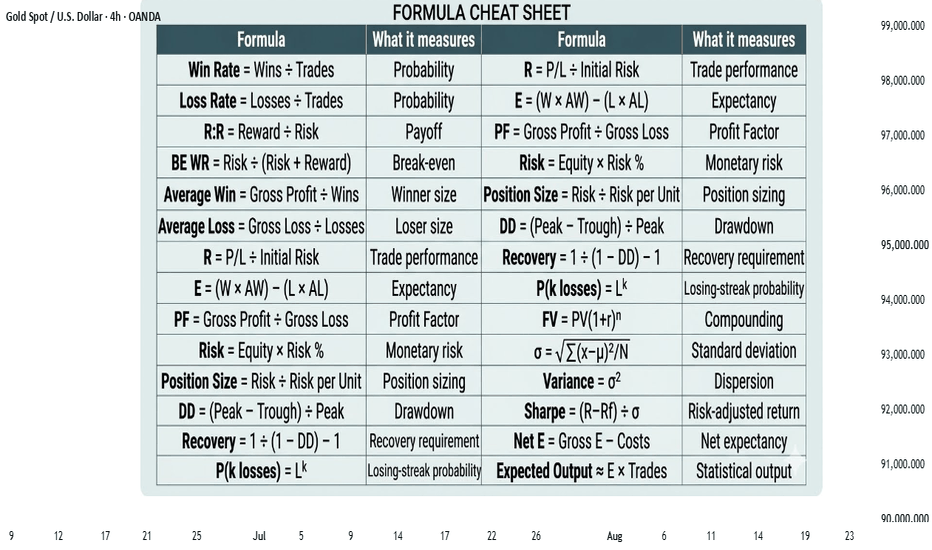
Making the numbers work.

Win rate, Risk : Reward, Expectancy, Position sizing & Compounding.

Here is the mathematics behind profitable trading.

1. WIN RATE

Win rate tells you how frequently a strategy produces winning trades.

Formula

Win Rate = Winning Trades ÷ Total Trades × 100

Example:

45 winners from 100 trades:
45%


2. LOSS RATE
Formula

Loss Rate = Losing Trades ÷ Total Trades × 100

If the win rate is 45%:

Loss Rate = 55%

Win rate and loss rate form the probability component of a trading system.

3. RISK-TO-REWARD
Formula

R:R = Potential Reward ÷ Initial Risk

Risk $100 to potentially make $300:

1:3

The payoff structure determines how much you need to win to overcome your losses.

4. BREAK-EVEN WIN RATE
Formula

Break-even Win Rate = Risk ÷ (Risk + Reward)

These figures assume no trading costs.

A 1:3 setup does not mean you only need to win 25% of your trades in real trading. Costs and the difference between planned and realised R matter.

5. AVERAGE WIN & AVERAGE LOSS
Average Win

Average Win = Gross Profit ÷ Winning Trades

Average Loss

Average Loss = Gross Loss ÷ Losing Trades

Example:

50 winners generate $10,000:

Average Win = $200

50 losers generate $5,000:

Average Loss = $100

These two numbers tell you what your winners and losers are actually worth.

6. R-MULTIPLE

R expresses every trade relative to its initial risk.

Formula

R = Profit or Loss ÷ Initial Risk

If initial risk is $100:

−$100 = −1R
+$100 = +1R
+$200 = +2R
+$300 = +3R

R allows performance to be compared across different account sizes.

7. EXPECTANCY

Expectancy combines probability and payoff.

Formula

E = (W × AW) − (L × AL)

Where:

W = win rate
AW = average win
L = loss rate
AL = average loss

Example:

45% win rate
Average win = $300
55% loss rate
Average loss = $150

E = (0.45 × $300) − (0.55 × $150)

E = +$52.50

The strategy can lose more trades than it wins and still have positive expectancy.

In R

E(R) = (W × Average Win in R) − (L × Average Loss in R)

45% winners averaging +2R and 55% losers averaging −1R:

(0.45 × 2) − (0.55 × 1) = +0.35R

That is the mathematical edge.

8. PROFIT FACTOR
Formula

Profit Factor = Gross Profit ÷ Gross Loss

Example:

$15,000 gross profit
$10,000 gross loss

PF = 1.50

A profit factor above 1 means gross profits exceed gross losses.

It should be evaluated alongside sample size and drawdown.

9. POSITION SIZING

The trade idea determines where the stop belongs.

Risk determines how large the position should be.

Formula

Risk Amount = Equity × Risk %

If:

Account = $1,000
Risk = 1%

Risk Amount = $10

A simplified position-sizing relationship is:

Position Size = Risk Amount ÷ Risk per Unit

Your position size should come from your risk not your confidence.

10. FIXED-FRACTIONAL RISK
Percentage-based risk automatically adjusts with account equity.

Formula

Riskₙ = Equityₙ × Risk %

At 2% risk:

$1,000 → $20

$1,500 → $30

$700 → $14

This makes risk proportional to the account rather than fixed in dollar terms.

11. VOLATILITY & ATR

A stop measured in absolute price distance does not represent the same market risk in every volatility environment.

Average True Range, or ATR, measures recent price-range behaviour.

A useful relationship is:

Position Size ∝ Risk ÷ Volatility

When volatility increases, maintaining the same monetary risk generally requires a smaller position.

Volatility should influence position size, not dictate your risk budget.

12. MAXIMUM DRAWDOWN
Formula

Drawdown = (Peak Equity − Trough Equity) ÷ Peak Equity × 100

If equity falls from $10,000 to $7,000:

30% drawdown

Drawdown measures the damage between an equity peak and subsequent trough.

13. LOSING STREAKS

If the probability of losing a trade is L, the simplified probability of k consecutive losses is:

P(k losses) = Lᵏ

For a 60% loss probability:

0.60¹⁰ ≈ 0.60%

This assumes independent outcomes and is therefore a model, not a prediction.

The important question is:

Can your account survive the losing streak your strategy can realistically produce?

14. RISK OF RUIN

Risk of ruin depends on:

Win probability, Payoff distribution, Risk per trade, Number of trades, Correlation & Definition of ruin

There is no single universal formula that applies to every trading strategy.

But the relationship is simple:

The greater the risk per trade, the greater the damage caused by a losing sequence.

A positive expectancy strategy can still fail financially when position sizing is excessive.

15. KELLY CRITERION

Kelly estimates a theoretical capital fraction for maximizing long-term geometric growth under specified assumptions.

For a simple binary payoff:

f = (bp − q) ÷ b

Where:

f = fraction of capital
b = net odds
p = probability of winning
q = probability of losing

Full Kelly can generate substantial volatility and drawdowns.

This is why fractional Kelly is often considered when applying the concept in practice.

16. COMPOUNDING
Formula

FV = PV × (1 + r)ⁿ

Where:

FV = future value
PV = starting capital
r = return per period
n = number of periods

Example:

$100 growing by 10% for five periods:

$100 × 1.10⁵

$161.05

The important feature is that each period starts with a different capital base. That is the mathematics of compounding.

18. THE $10 → $90,000+ MODEL

This is where the mathematics becomes interesting.

Starting capital:

$10

Target:

$90,000+

For 10 equally performing setups:

Final Balance = $10 × (1 + r)¹⁰

To reach approximately $90,000:

r ≈ 149% per setup

because:

$10 × 2.49¹⁰ ≈ $90,000

But a real 10-setup model does not need every setup to produce exactly the same return.

The general equation is:

Final Balance = $10 × ∏(1 + rᵢ)

Each setup can therefore have a different return.

The mathematical progression is:

$10

→ Setup 1

→ Setup 2

→ Setup 3

→ Setup 4

→ Setup 5

→ Setup 6

→ Setup 7

→ Setup 8

→ Setup 9

→ Setup 10

→ $90,000+

This is a mathematical compounding model, not a guaranteed trading outcome.

Losses, spreads, commissions, slippage, execution limits and changing market conditions can prevent the model from being achieved.

18. GEOMETRIC RETURN

Compounding makes the sequence of returns important.

Suppose an account gains 10% and then loses 10%.

The arithmetic average is:

0%

But the account becomes:

$100 × 1.10 × 0.90 = $99

The actual result is:

−1%

This is why average return alone can be misleading.

The sequence matters.

20. SAMPLE SIZE

Suppose a trader wins:

8 out of 10 trades

Observed win rate:

80%

That does not prove the strategy has an 80% true win rate.

A larger sample provides more information about:

Win rate
Average R
Expectancy
Drawdown
Losing streaks
Return distribution

Ten trades can show what happened. They cannot reliably establish what will happen long term.

20. STANDARD DEVIATION & VARIANCE

Standard deviation measures how widely returns vary around their mean.

Formula

σ = √

Variance is:

Variance = σ²

Higher dispersion means greater variability in outcomes.

These measures become important when evaluating the stability and risk of a return stream.

21. SHARPE RATIO

A return should be considered relative to the variability required to achieve it.

Formula

Sharpe Ratio = (Return − Risk-Free Rate) ÷ Standard Deviation

Two strategies can produce the same return while exposing the trader to very different levels of variability.

Return alone is incomplete.

22. CORRELATION & PORTFOLIO RISK

Trading five instruments does not necessarily mean having five independent positions.

Correlation measures how return series move relative to each other.

Approximately:

+1 → strong positive relationship

0 → little linear relationship

−1 → strong negative relationship

If five trades are highly correlated, their combined exposure can behave like one much larger directional position.

Therefore:

Individual trade risk ≠ total portfolio risk

23. TRADING COSTS

A theoretical edge must survive real execution.

Formula

Net Expectancy = Gross Expectancy − Trading Costs

Costs can include:

Spread, Commission, Slippage, Financing or swap & Other transaction costs

A strategy that looks profitable before costs may not remain profitable after costs.

The edge has to survive friction.

24. MAE & MFE
Maximum Adverse Excursion — MAE

Measures how far a trade moves against you before closing.

It can help determine whether:

*Stops are too tight
*Normal volatility is being mistaken for invalidation
*Winners frequently experience adverse movement
*Maximum Favorable Excursion — MFE

Measures how far a trade moves in your favour before closing.

It can help determine whether:

*Targets are too ambitious
*Winners are being closed too early
*Realised profits are much smaller than available price movement

Together, MAE and MFE show what happens inside the trade, not just at the entry and exit.

25. REALISED R

A trade may be planned as a 1:3 setup.

But if it is repeatedly closed at +1R, the realised result is not 3R.

Therefore:

Measure realised R, not just planned R:R.

Your trading journal should tell you what your strategy actually produces.

26. MEAN, MEDIAN & DISTRIBUTION

Consider:

+1R, +1R, +1R, +1R, +20R

Mean:

4.8R

Median:

1R

The mean is heavily influenced by the single +20R outcome.

This is why traders should examine the distribution of returns, rather than relying on one headline statistic.

Ask:

Where do the returns actually come from?

27. MONTE CARLO ANALYSIS

Historical trades occurred in one particular sequence.

Monte Carlo analysis can simulate alternative sequences from historical results.

It can help examine:

*Potential drawdowns
*Losing streaks
*Equity-curve variation
*Range of possible outcomes
*Sensitivity to trade sequencing

It does not predict the future.

It asks a different question:

What could happen if the same statistical characteristics appeared in a different sequence?

28. EXPECTED OUTPUT

Once expectancy is known, opportunity becomes important.

Formula

Expected Profit ≈ Expectancy per Trade × Number of Trades

If expectancy is:

+0.35R

and the strategy produces:

200 trades

then:

Expected output = +70R

This is a statistical expectation, not a guaranteed result.

A strong edge with very few opportunities may produce less total output than a smaller edge expressed frequently.

29. EDGE DECAY
A historical edge is not a permanent law.

Market structure, volatility, liquidity, competition and execution conditions can change.

If a strategy historically produced:

+0.40R

future expectancy may be lower, higher or negative.

Therefore, performance must be monitored continuously.

An edge must be demonstrated, not assumed.

THE MATHEMATICAL FRAMEWORK

A trading system can ultimately be reduced to a chain:

Probability

↓

Payoff

↓

Expectancy

↓

Position Size

↓

Execution Costs

↓

Variance

↓

Drawdown

↓

Compounding

↓

EQUITY GROWTH

But the same mathematics works in reverse.

*Losses reduce the capital base.
*Drawdowns increase the percentage return required for recovery.
*Aggressive position sizing increases the impact of variance.

Therefore:

Compounding is powerful. Risk determines whether you survive long enough to use it.

The $10 → $90,000+ model is a mathematical demonstration of compounding across 10 setups.

It is not a promise that the market will produce those returns. the most important thing is :

Probability + Payoff + Positive Expectancy + Controlled Risk + Sufficient Opportunity.

A strategy can lose frequently and still make money, A strategy can win frequently and still lose money. The difference is in the mathematics.

put together by : @currencynerd